Revision to GAFTA sampling rules
Since I started in this business in the 1990s, much of my work has been with grains and animal feedstuffs. Huge quantities of grain and feeds are traded by sea, and it is no exaggeration to say that this trade is necessary to feed the world. It is a widely quoted statistic that 80% of the world trade in grain and animal feeds is by means of GAFTA contracts.

GAFTA is an acronym for the Grain and Feed Trade Association. I’m pleased to be able to say that Sheard Scientific is a member of GAFTA.
Trade based on GAFTA contracts usually adopts the concept that the definitive and “final” check on the quality of the goods being traded occurs at the time of loading. This enables a degree of certainty to those participating in the trade, but the concept does require reliable sampling and analysis. That sampling is required to be carried out according to GAFTA 124 sampling rules.
I may write in more detail about sampling as a general topic in a later post (time allowing!), but suffice it to say here that representative samples by definition are to represent the average properties of the parcel of cargo being sampled. Since those samples have to be much smaller in size than the cargo they are drawn from, they have to be drawn in a manner which gives equal statistical chance for any given particle in the cargo being sampled to be in the working/drawn sample.

The purpose of GAFTA 124 is to set a standard for how that is to be carried out, how the integrity of the samples should be preserved, and what should be done with them. Whilst the official scope of GAFTA 124 is in reference to the GAFTA sales and purchase contracts, to ensure quality parameters are properly and reliably assessed when a cargo is traded, it is in my experience so commonplace as to be universal that they are used as a benchmark “gold standard” for sampling of cargoes where there is a dispute – in circumstances where there has been transit damage, for instance. The GAFTA sampling rules don’t necessarily suit all such circumstances, but they are always where surveyors and experts start when considering how to sample average parameters of bulk grain or feeds.
Bearing that in mind, a change to the GAFTA 124 rules is potentially big news, and so I read with interest when I received notification of the changes. There have been substantial changes to the GAFTA 124 rules over the years I have been working in this industry – when I first started, in all cases sublots were 500MT in size – meaning dozens of sublots for a moderate sized vessel. That has long-since been changed so that the selection of sublot sizing scales with the overall consignment quantity.
One change being introduced in the new version of the rules is that there is greater clarity regarding the numbers of individual bags from which samples must be taken when bagged goods are being sampled.
Paragraph 9.1.8 now contains the following text, seemingly to ensure that all are made aware of the status of “certificate final” provisions and that sets of samples reserved for arbitration are not to be used to overturn compliant load port certification.
Arbitration samples drawn for goods traded on contracts stating ‘Quality (Certificate) Final’ at loading or at discharge cannot be used to challenge the quality specifications which are included in the ‘Quality (Certificate) Final’ certificate, unless otherwise determined by arbitrators or Board of Appeal.
But to my eyes, the biggest change is in the selection of laboratories. Again, back when I started this work, in the case of any disputes or disagreements, specific laboratories were to be used as “referee” laboratories. In recent years there have been four designated as referee laboratories and their identities were written into GAFTA 124. The four reference laboratories were undeniably “household names” to all in the grain trade, and will no doubt continue to be used as reliable grain testing facilities. However, it is now the case that any GAFTA-approved laboratory can serve this purpose as all approved labs are considered equivalent.
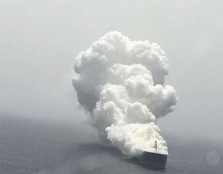
Direct Reduced Iron – one of the most unpleasant cargoes out there
It really is. But why?
This article will, I hope, give you some idea why. What it won’t do is catalogue the different types of DRI you might encounter and what the requirements are to handle or carry them safely. That might be a future article, but this one is meant to explain the science underlying DRI and what gives rise to its hazards.
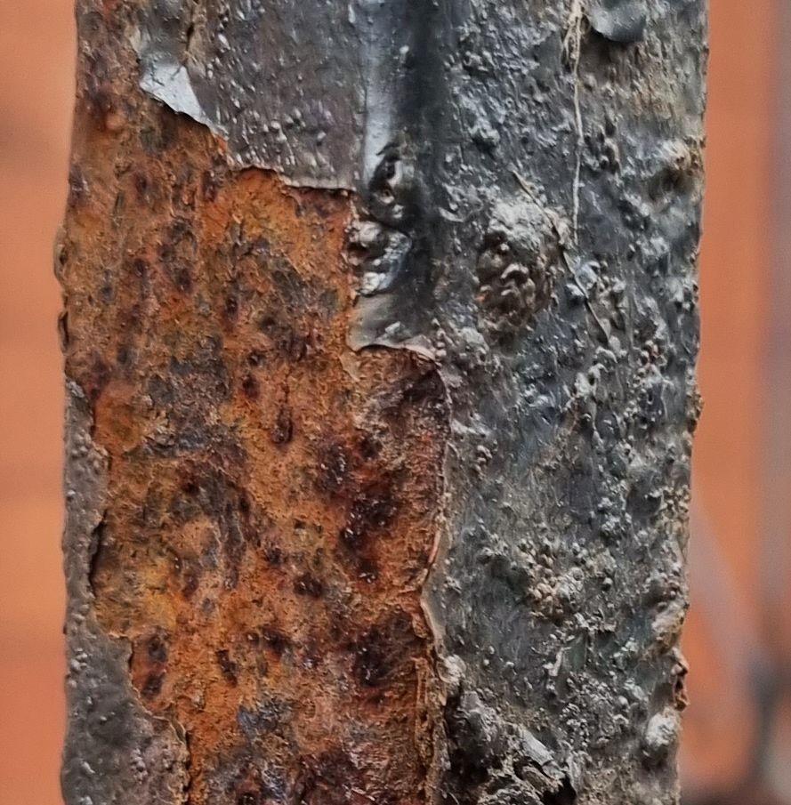
Iron is a very familiar substance – we make all sorts of things out of it or things based on it. Steel structures are found in buildings, cars are made from steel, we have iron railings and gates, and there are many many more examples. There’s a property in common with many of these man made objects, and that is that they rust if you don’t prevent it. Rusting is a very familiar example of an oxidation reaction. Iron plus oxygen becomes iron oxide, one type of which is the familiar red/brown rust we see on iron railings and the steelwork of older cars.
There is lots of iron around in the earth’s crust – that is because the familiar isotopes of iron are, in nuclear physics terms, the most stable substances known. Nuclear stability arises from the lack of tendency to undergo nuclear fission or nuclear fusion. Those two processes release energy from the nucleus when that nucleus splits (fission) or merges with another (fusion). Splitting a nucleus of iron will always cost energy, similarly trying to fuse iron with other nuclei will also absorb energy. Thus iron nuclei are highly stable, and form a substantial proportion of the end-products of the explosions known as supernovae and in other stellar processes. As these are where the elements making up the earth (including those in you and me!) are formed, the presence of large amounts of iron (and also nickel) in the earth’s crust and core is unsurprising. But I digress.
Iron is a moderately reactive metal and is always found in nature combined with other substances as ores. Iron ore might contain iron oxides, iron sulphides, or other forms.
Production of metallic iron from naturally occurring iron ores was first carried out by mankind over 3000 years ago. It was such an important development that the term “iron age” describes the period when iron became available for use. Early furnaces could not reach the melting point of iron and produced a form of the metal known as a “bloom”. Later furnaces used forced air draughts to reach higher temperatures and are known as blast furnaces. These produce molten iron, known as “pig” iron which can then be used in steelmaking.
Ironically (geddit?) DRI has more in common with obsolete bloom iron than more modern blast furnace forms. Consider an ore which is mostly iron oxide. Chemically, this is an example of an ionic material. The iron atoms are present as positively charged iron ions, and the oxygen atoms are present as negatively charged ions. In a piece of solid iron ore, between each pair of adjacent iron atoms is found an oxygen atom, and vice versa.
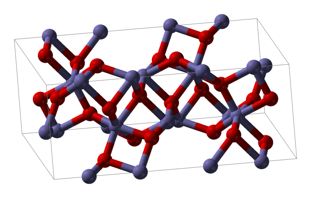
Direct reduction involves the removal of the oxygens without melting the feedstock. Typically the feedstock is pelletised iron ore, each pellet being roughly 1cm in diameter. When the oxygen is removed from the pellet without melting the pellet, the shape and size is retained but the locations which used to have oxygen atoms in them now have gaps. These tiny gaps are all interconnected and the resulting pellet of DRI is extremely porous. It has a huge surface area yet weighs less than the pellet it was made from. Once reduced, it looks very much like a malteser (without the chocolate coating).
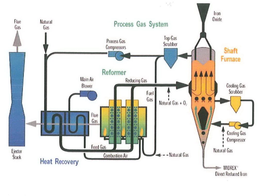
I’m going to refer to DRI made by the MIDREX process, which is made in a shaft furnace. The reducing agent (i.e. the material used to remove the oxygen) is hydrogen and carbon monoxide made from natural gas. Natural gas is also used to heat the furnace, but because the ore is not melted, less heat is required than other furnace types, meaning that the DRI process is relatively energy-efficient. The need for natural gas to heat the furnace and provide the reducing gas means that DRI plants are usually found in locations where gas is plentiful and relatively inexpensive.
A parameter often quoted in the context of DRI is % metallisation. This is the percentage of the iron in the pellet which is present as free metallic iron rather than oxides. With modern DRI facilities, metallisation will be 95% or so. This iron can be used directly in steelmaking.
Because DRI production tends to take place where the natural gas is, it is often then carried by sea to a steel mill. That is unfortunately where some of the problems arise.
All of the problems associated with DRI come about because of the physical form that iron is in. A lump of iron can rust at its surface. That rusting usually involves water, and rusting by sea water is more rapid than with fresh water. Rusting to a cargo of DRI, especially if wetted by sea water ingress, can damage the cargo by allowing parts of it to revert to iron oxide. Loss of cargo value is undoubtedly something a shipowner will want to avoid, but there are much more immediate problems a vessel is likely to face if DRI becomes damaged on board.
Rusting is an oxidation reaction, and like all oxidative reactions, involves the release of heat. Quite a lot of heat in chemical terms, but we don’t notice a rusty car or iron railing getting hot as it rusts. Why not?
The answer is that the rusting only happens at the exposed surface of the railings or car structure, and does so slowly enough that any heat generated is immediately lost to the atmosphere. There’s never a temperature rise.
In contrast, a pellet of DRI has a huge surface area – some estimates suggest that a pellet of DRI has a surface area 10000 greater than a lump of solid iron. That means that when the DRI is freshly produced it has 10000 times the capability of reacting with oxygen and rusting. That’s one reason that DRI behaves differently to a lump or a gate made of iron.
The other hugely significant property of DRI is that, like most bulk cargoes, it is a poor conductor of heat. That might be a little surprising to hear as there is nothing there other than iron, and metals conduct heat, don’t they?
A block of iron does indeed conduct heat. A bulk made up of spheres made out of iron does not conduct very well because the contact area between adjacent spheres is small and thermal contact is poor. A bulk made up of DRI, in which much of the surface area is space rather than metal conducts heat very badly indeed.
That means that where (for example), sea water enters a bulk stow of DRI, the first thing which happens is that the wetted iron rusts. Fresh water will cause rusting but sea water makes it happen much more rapidly. The heat released by the rusting reaction, which for most of the forms of iron we encounter everyday is lost immediately, does not get conducted away and makes the temperature rise locally where the DRI was wetted.
As the temperature of the iron at those points within the stow rises, it may reach a high enough temperature that the iron can react directly with the oxygen in the hold (if there is any!). This isn’t rusting any more but is direct oxidation. The higher the temperature gets, the more rapidly the reaction goes.
If there is a ready supply of fresh air/oxygen, a DRI cargo can heat to several hundred degrees Celsius and will keep going. Whilst the rate of heat conduction within the bulk is low, it isn’t nil, and gradually the volume of DRI involved with what is now referred to as a “metal fire” increases. It may pass from hold to hold through a bulkhead. It may overheat fuel in adjacent tanks.
As I said, this article is not going to go into detail about what the different types of DRI are and how they should be carried. I will say, however, that one of the main tools in the arsenal of a vessel carrying DRI is the ability to exclude oxygen from the stow. This may be enough to prevent a fire in the first place, or it may help in keeping a situation under control so the vessel can safely reach a port where the problem can be dealt with. Nitrogen gas is used to inert holds carrying some types of DRI precisely for this purpose. Unfortunately, the more commonly found carbon dioxide inert gas is not suitable.
When DRI gets to high temperatures, it becomes a very difficult commodity to deal with. Hot DRI really loves oxygen, and will do almost anything to get it. Nitrogen is effective in stabilising where the hatches are closed, but oxygen will inevitably get into the stow during discharge. Temperatures can get very high indeed and there can be a risk to the vessel itself.
The only recourse available to assist during the discharge of a problem DRI cargo is to use water. Even that is fraught with difficulty. There are multiple problems. Firstly, problematic DRI can be at several hundreds of degrees or more. Initial amounts of water will simply be boiled off as steam. You have to be able to put water in there quicker than the DRI can boil it off.
Next problem is that water is H2O, and that O is of course oxygen. Hot DRI can satisfy its need for oxygen directly from the water you are pouring on it. The DRI takes the O, creating more heat and leaving the H2. This is hydrogen gas, very volatile and highly flammable. Be ready for whooshes of flame from the hydrogen, assuming you successfully avoid an explosion.
And then there is the fact that you are putting water, possibly even sea water, onto DRI. Any thought you might have had of salvaging any of the cargo is probably history by now, but there is a very real problem of creating further heating in stockpiles (hopefully ashore) from wetting by extinguishing water.
If all of that wasn’t enough, the final insult is that that the resulting oxidised DRI will weigh about 30% more than the DRI cargo you started with. Anecdotally, problems involving the collapse of quay structures have been caused by underestimating the weight of the reoxidised cargo.
Phew. If you are going to carry DRI, it really is very important that you don’t have a problem. But DRI can cause difficulties even when there isn’t an emergency/fire situation. What might they be?
Inevitably during loading and discharge, dust is created. That dust is metallic iron. The IMSBC Code warns about the need to remove accumulations of dust as quickly as possible. I have seen first-hand what happens if you don’t or can’t. Accumulations of DRI dust embed themselves into paint and then rust. This is not only unsightly but it can cause significant operational problems. The Code also warns about the potential for damage to radio and other aerials/antennae.
All in all, carriage of DRI is not something to be embarked upon without a great deal of preparation and care. At Sheard Scientfic, we have first-hand experience of dealing with carriage and consequences of carriage of DRI and can assist our clients with this highly problematic material.
Biotechnology and GMOs – Part 2 – what is PCR?
In recent weeks, a number of P&I Clubs have circulated an information document kindly produced by Istanbul Correspondents Vitsan. This document warns that Turkish Courts have banned the import of distillers dried grains & solubles (DDGS) cargoes containing a particular genetically modified maize variety (MON810, more about that later).
The document warns that paperwork needs to be in order regarding shipments of DDGS being imported to Turkey. It seems likely that some form of testing on arrival may take place, and that is going to use a test known as PCR. But what is it?
PCR is the Polymerase Chain Reaction. There you go – shortest post ever!
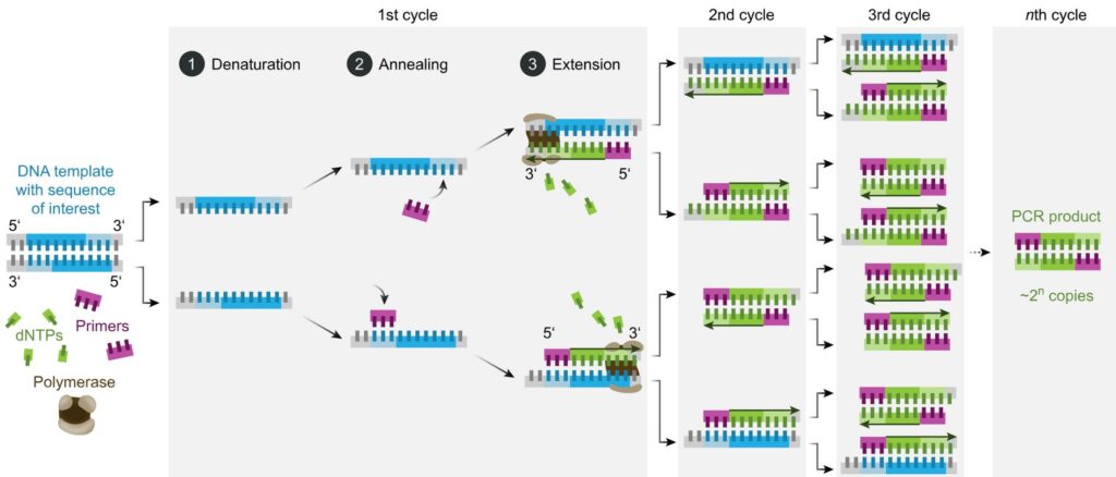
Ah, you want to know how it works and what it does? OK, step this way. All through the weekly COVID Government updates, we heard the experts and Ministers use this acronym repeatedly. Before the advent of cheap lateral flow tests, it was the only way to establish if someone had that infection. It remains the way of investigating which variant of the virus an individual has, demonstrating when new variants appear, and tracking the spread of those variants. Whenever you see DNA testing referred to on CSI/forensics TV shows, PCR is the technique they are applying.
As a tool, it has revolutionised molecular biology, and it is difficult to imagine modern genetics being developed without it. That is remarkable bearing in mind it was only developed in the 1980s.
There’s no substitute to understanding the basics of how it works. Fundamentally, it selectively reproduces and amplifies a specific segment of DNA, if it is present.
I discussed in a previous post what DNA is and how it codes for information. DNA exists as a double-helix, with the gaps between the backbones occupied by base pairs AT, TA, GC and CG. This is referred to as double-stranded DNA. Each sugar backbone molecule (dexoyribose sugar) is joined to the next sugar in the same way – carbon 5 on one molecule is joined to carbon 3 on the next. The two helices run in the opposite directions and are joined together by the base pairs.
When DNA is heated up, the two strands separate. This is sometimes called “melting”, and it happens at a temperature of around 94-98oC. The two strands, now separated from each other, both contain the full genetic information the DNA coded for. That is because each A on the top strand was originally paired with a T on the bottom, each G with a C and so on.
This means that if there was a mechanism of adding new bases and deoxyribose sugars to a single strand of DNA, the full double stranded molecule could be recreated. This is what happens in cellular division in real life – the double-stranded DNA is separated into two single strands (not by heat in a cell, though!) and the cell then creates new matching strands leaving it with two identical DNA molecules. This replication process is where errors can arise resulting in genetic mutations, but this article isn’t the place to go into that.
So, inevitably, cells already have the equipment to synthesise a replacement strand to convert single-stranded DNA to double-stranded. This equipment is an enzyme known as a DNA polymerase. It needs a supply of free bases and dexoyribose sugar backbones to work.
It also needs something else. DNA polymerase requires a segment of double-stranded DNA in order to start. Once it has started, it will continue literally up the existing strand of DNA, manufacturing a complementary strand to produce double stranded DNA. Think of it as being like a zipper – you have to start a zipper by aligning the starting pieces. DNA polymerase works along like a zipper but it manufactures one side of the zip as it goes.
In a PCR reaction, short segments of single stranded DNA sequences known as primers are put into the reaction vessel. These are designed to be a perfect match for part of the DNA being tested for. Two primers are used – one matches a sequence on one strand of DNA, the other matches a sequence on the other.
In order for the primers to settle and bind on the sequences they match, the temperature has to be lower than the 94-98oC I mentioned above to separate double-stranded DNA. Typically this happens around 50-65oC. The primer sequences then act as the starter for the DNA polymerase to start and zip from.
Most DNA polymerase enzymes are not sufficiently thermally stable to survive being heated to 94-98oC in the first step. Such enzymes would need to be added, and then the “zipping”/elongation stage is usually run around 72-75oC. However, a crucial discovery for the development of PCR was the existence of a DNA polymerase from the organism Thermus aquaticus, which can survive at the 94-98oC required to denature DNA. This enzyme is known as Taq polymerase after the organism it was extracted from.
PCR is a reaction run in cycles. A reaction vessel is used into which are placed the DNA to be tested, primer sequences, base pairs on deoxyribose sugar backbones, and Taq polymerase. The reaction proceeds as follows (leaving out initial and final temperature changes which are significant but outside the scope of this article).
- Denaturation. 94-98oC for 20-30 seconds. Long enough to separate the double-stranded DNA to single stranded but not long enough to destroy the Taq enzyme.
- Annealing. 50-65oC for 20-40 seconds. In this time the primers bind to DNA sequences on the target DNA, if those sequences are present. Choice of primers and temperature are crucial – see below.
- Elongation. 72oC. Required time varies. In this period the Taq polymerase synthesises a new strand of DNA starting at a primer and running onwards until it reaches the end of the DNA strand or runs out of time.
- Repeat
The reaction is controlled by the temperature – thus the reaction tubes are placed in a machine which cycles the temperature through the regime listed above. Each full cycle takes a couple of minutes. In an hour or so, it is straightforward for 30 cycles to be run without any more reactants needing to be added to the vessel or any other intervention.
As mentioned above, PCR is used to amplify in a selective manner a particular fragment of DNA. Assume that we are testing for the presence of MON810 maize DNA, and that the sample being tested does indeed contain that DNA – but only one molecule of it. (Potentially bad news if you are importing that maize to Turkey). The denaturation step will create two single-stranded segments of DNA from the extracted maize sample. These will not be the same but one will be effectively the reverse/mirror of the other. One primer must be designed to be a match/complement to a DNA sequence on one strand, and the other primer to a different area on the second strand. They bracket the DNA sequence to be amplified.
On the first cycle, one primer will bind to each strand of the sample DNA, and those will be elongated in step 3. Note that the DNA sections extracted from the maize sample might be very long indeed. The elongated copies made in this first step 3 will start at a primer (because that is how Taq polymerase works) and will extend for some distance until the point where the polymerase ran out of time in step 3.
On the second cycle things become interesting. Denaturation will produce four single-strands of DNA. Two of these will be the original ones from the sample (of whatever length they were) but the other two will start with one of the primers and will then be of random length. Call the two primers P1 and P2.
The strand synthesised in the first reaction starting with P1 doesn’t contain a sequence P1 can bind to – so only P2 can bind. Similarly, the strand which started with P2 in the first cycle will then bind with P1. Elongation in the second cycle will produce double sided DNA from all four single strands. Two of these (the ones produced from the synthesised segments in cycle 1) will have a new segment synthesised which starts at P1 and stops at P2. That is the desired amplification product.
At the end of the second cycle, we are left with four double stranded segments of DNA. When denatured at the start of the third cycle, six of these (i.e. the two original DNA strands, the two synthesised in cycle 1, and two of the four synthesised in cycle 2) are what is known as variable length strands. The other two however are exactly the same length as each other, and that length is the number of DNA base pairs between the sequences in the original DNA which bind to P1 and P2.
This might not sound so great, as we have three times as many DNA fragments of variable length than the specific sequence we were intending to multiply.
However, at the end of this third cycle, we have 16 strands of DNA. Eight of these are variable length fragments (two new variable length fragments were synthesised in cycle 3 from the original sample DNA). However, the other eight are exactly the same length – each starts at the location of P1 and runs to the location of P2.
At the end of the fourth cycle we have 32 strands of DNA. Ten are variable length, but all of the rest are exactly the same – starting at P1 and ending at P2.
However, now run the reaction cycle a further 29 times. You end up with a couple of hundred variable length fragments and over 1,000,000,000 (one US billion) identical copies of a fragment exactly the length bounded by P1 and P2. The enormous quantities of exact length fragments completely swamp the variable lengths fragments.
The resulting contents of the reaction tube are then visualised in some way so that the results can be understood. They might be separated on a gel – this is how the charts are produced showing the characteristic lines we see in DNA results. Each line is an amplified fragment – a fragment bounded by two specific primers. These amplified fragments, even from a tiny original amount of DNA, are present in such enormous numbers they are readily detected and visualised.
To return to our example, if the sample of maize DNA didn’t contain a fragment from MON810, that fragment couldn’t be amplified, and that “line” would be absent on the chart.
Everything then depends on the selection of suitable primers (and to some extent, the fine-tuning of the temperatures used in the PCR cycles). The primers need to be long enough that there is no chance of those sequences being found elsewhere in the maize genome, and they need to be short enough to bind with the target DNA during step 2 of each cycle – if they don’t then there is nothing for Taq polymerase to zip from.
As an example, the EU reference test for MON810 uses the following primers
- P1 – TCGAAGGACGAAGGACTCTAACGT
- P2 – GCCACCTTCCTTTTCCACTATCTT (reverse strand)
This test is known as an “event specific” test because primer P1 binds to a sequence on the maize parent plant whereas P2 binds to a sequence on the inserted gene – i.e. the fragment to be amplified contains a section of DNA from the maize and a section from the insert, it flanks the genetic insertion. Thus this test only detects MON810, it doesn’t (for instance) detect other GMOs which contain the same inserted DNA.
More on the use of PCR to detect GMOs in relation to shipping in a later article.
For now, I will offer some comments on the generalities of using PCR and the MON810 variation.
The enormous specific amplification provided by even 30 cycles of PCR means that very tiny amounts of DNA can be detected. Provided the primers are appropriately selected, the test is wholly specific – it only detects the sequences it was designed to detect. There are off-the-shelf primer kits available for commercially produced GMO plants. Thus an event specific test can be anticipated to exist for any GMO likely to be found in a real world shipment.
As long ago as 1999, methods for detection of GMOs were being studied in the context of commercial commodities. This is because of the fear which has existed for some time of “Frankenstein foods” and other issues relating to escape of modified material into the natural environment. One particular study looked for a specific GMO soya type (commonly known as Roundup-Ready soya) not in samples of soya but in wheat bread. Soya was only in the bread as a minor component of the baking improver/powder. Despite the steps making up the dough production and baking, GMO soya was readily detected in loaves produced using that baking aid – even though the soya made up only 0.4% of the dough mix. In that study, commercial baking aids were also tested, and in 2 out of 15 off-the-shelf products tested the GMO soya could be detected in the baked bread. Back in 1999!
And so, by a roundabout route we return to maize and MON810. MON810 is quite an early GMO product of the Monsanto company. It was made by inserting DNA from a bacterium Bacillus thuringiensis. In the bacterium this produces a toxin which affects certain butterflies and moths, some of which as larvae damage maize plants. The idea of the modification was that the maize plants would produce the toxin, and that would serve as a control over the larvae, thus reducing the need to apply pesticides. MON810 has been commercially very successful and has been very widely planted. The modification was produced by firing projectiles containing the bacterial DNA at plant cells.
MON810 has been the subject of some controversy. It has been suggested that the use of this variety can be responsible for the death of bee colonies. As far as I am aware, this allegation, or indeed any other specific allegations of harmful effects from MON810 has not been proven.
As stated above, the EU test for MON810 is event specific and will detect very small amounts of the GMO. Even a fragment from a MON810 plant will, if it ends up in a sample sent for testing, lead to a positive result. I note that the Vitsan circular relates to imports of distillers dried grains & solubles (DDGS) – not the maize itself. DDGS is produced from harvested maize by a series of industrial steps, but by analogy to the baking powder/bread study referenced above, these processes are not likely to prevent detection of modified genetic material if MON810 was present in the original unprocessed maize.
I note that Vitsan have specifically clarified that a different product, NK603xMON810 maize is allowed to be imported, provided it is referenced as MON-00603-6xMON-00810-6. The “x” in this designation identifies that this is a so-called “stacked trait”. This means that the maize variety MON-00603-6xMON-00810-6 carries the properties of MON810 and the properties of MON603. The GMO event 603 is a Roundup-Ready variety of maize. Thus the stacked trait is resistant to the herbicide Roundup (glyphosate) and also produces the bacterial toxin to kill the larvae mentioned above.
Often, but not always, stacked traits are produced by conventional genetic crossing techniques. If this is done, and plants which express both traits are selected for, then BOTH events will be present in the marketed product. Thus a test for event MON810 will be positive, as will a test for event 603. It is not clear to the writer what undesirable properties could exist in MON810 which are not also present in MON-00603-6xMON-00810-6. I do not have sufficient data yet to say whether MON-00603-6xMON-00810-6 will test positive in an event specific test for MON810.
It appears likely that there may be difficulties with testing surrounding verification for this regulation – i.e. cargoes of DDGS may be rejected when they should not be. The presence of genetically modified material is not something which can be detected by the naked eye nor even field testing. It requires sampling and laboratory analysis, and there is always scope for a misleading result.
A new Code – Part 2
So what’s new?
Starting with the Supplement, there is a new document entitled “Guidance for conducting the refined MHB (CR) test”. MHB materials are those with hazards which are not to be found in the IMDG Code as they are only considered hazardous when in bulk form. The application of MHB has changed in approach in recent years, and I will write about that separately.
The new document to be found in the Supplement relates to extending the scope of a UN Standard test (known as the C1 test) to apply to examining the corrosivity of bulk solids. The document notes that the C1 test in its standard published form does not give reliable results for bulk solids. The new guidance runs to several pages and is in effect a modification or adaptation to the C1 test enabling it to be conducted on bulk solids. This fortunately isn’t something most vessels will need to encounter.
Also in the Supplement is a new version of the document issued as circular 1395. This document contains “Lists of solid bulk cargoes for which a fixed gas fire-extinguishing system may be exempted or for which a fixed gas fire-extinguishing system is ineffective”. This document has been updated to include the materials to be found in the new Code schedules – see below. I note that this document relates to what are usually referred to as CO2 systems on ships. The CO2 system is frequently one of the first tools reached for by vessels undergoing a fire emergency. The first list in this document is made up of materials which are deemed very unlikely to support a fire. The second (for which a CO2 system is ineffective) is entirely made up of materials which are chemically inorganic nitrates. These are oxidising agents. As CO2 works by excluding oxygen and thus suppressing combustion, it is of no use for a cargo which contains its own oxidising agent.
Turning now to the main Code, a change which is really a matter of housekeeping from previous editions is the embedding of the concept of dynamic separation in the definitions and wording of parts of sections 1-13 of the Code (i.e. the bit before the appendices start). If you read my introduction to liquefaction, you may recall that dynamic separation as a phenomenon had been described in the new bauxite fines schedule. That schedule is of course to be found in Appendix 1 of the Code. No definition of dynamic separation existed in the sections of the Code discussing liquefaction, nor was there any wording to make it clear that Group A properties included both liquefaction and dynamic separation. Now there is.
The heading of Section 7, for instance is now “Cargoes which may liquefy or undergo dynamic separation“, whereas it was previously “Cargoes which may liquefy“. Similarly, the tests in Appendix 2 are now (all) tests for “materials which may liquefy or undergo dynamic separation.“
There is now a definition of the term “dynamic separation” itself, which is that
Dynamic separation means the phenomenon of forming a liquid slurry (water and fine solids) above the solid material, resulting in a free surface effect which may significantly affect the ship’s stability.
IMSBC Code definition of dynamic separation, 2022 Edition
This is the Code catching up with itself – the 2020 edition contained a schedule in an appendix which outlined a hazard which wasn’t defined in the Code itself. It is now very clear that dynamic separation and liquefaction are both to be taken as examples of Group A cargo behaviour. The procedure for preventing them is the same – Group A cargoes must be shipped at a moisture content below the determined Transportable Moisture Limit (TML).
Bearing that in mind, the distinction between liquefaction and dynamic separation only becomes significant when a cargo misbehaves. The emergency measures taken by a vessel may need to take into account whether the cargo is considered to be undergoing liquefaction or dynamic separation, but the normal routine handling and carriage does not.
Finally, I will turn to Appendix 1 – in this we find some new schedules and one commodity re-classified.
LEACH RESIDUE CONTAINING LEAD. This is a new schedule. It relates to solid residue produced during zinc extraction. Sulphuric acid is used to dissolve the zinc-bearing part of the ore or concentrate. What is left may contain lead (resulting in toxicity) and may be corrosive because of residual sulphuric acid. I note that this schedule is MHB TX and CR – the CR corrosive solid MHB hazard will require the new modified corrosivity test to be found in the Supplement. A Group A cargo on account of its particle sizing (granular), and a Group B cargo on account of the two MHB hazards.
CLAM SHELL. Another new schedule. Other than noting that it is Group C and relates only to whole clam shells, I have nothing to say!
SUPERPHOSPHATE (Triple, granular). This is a replacement schedule. In the previous edition of the Code, TSP (as it is usually known) was listed as a Group C cargo. The new schedule is a Group B schedule on account of it being a corrosive solid MHB. I note again that this requires the application of the new test to be found in the Supplement. TSP is the “ultimate” in a series of fertilisers obtaining fertilising phosphorous content (the P of NPK) manufactured from phosphate rock. Phosphate rock contains insoluble calcium phosphate, which is brought into solution by reacting with an acid. Sulphuric acid can be used which results in superphosphate. TSP has the highest amount of phosphorus in it, and it is made by reacting phosphoric acid with phosphate rock – the resulting material has phosphorus from both the phosphate rock and the phosphoric acid. Residual acidity results in the MHB CR designation.
… and finally, AMMONIUM NITRATE
There were four schedules for ammonium nitrate and material derived from it in the 2020 Code. They were
- Ammonium nitrate UN1942
- Ammonium nitrate based fertiliser UN2067
- Ammonium nitrate based fertiliser UN2071
- Ammonium nitrate based fertiliser (non-hazardous)
Of these, the “non hazardous” version was Group C and the first three were Group B cargoes. Note that ammonium nitrate in conjunction with combustible material such as fuel oil is highly explosive. One of the requirements to be considered non-hazardous was that the material passed the UN standard test known as the “trough test”. I wrote about this test and some of the problems arising from it earlier this year. I commented that the trough test did not fully reproduce the hazard of self-sustaining decomposition meaning that cargoes which were tested and certified as “ammonium nitrate fertiliser (non-hazardous)” could give rise to serious incidents.
I have, over the years, been consulted many times regarding proper classification of materials containing ammonium nitrate. I suspect the new provisions, whilst being technically more complete and consistent than the previous version, will also result in queries. That is because they are even more complicated.
In the new Code, 2022 edition, we now have (in the order they appear in the Code)
AMMONIUM NITRATE UN1942. This schedule is unchanged from previous versions which covers ammonium nitrate itself. It is a Group B schedule, Class 5.1 oxidiser and is an extremely hazardous substance. The schedule sets very strict limits on the amounts of combustible material.
AMMONIUM NITRATE BASED FERTILISER UN2067. This is also Group B, Class 5.1 and is carried over from previous versions. There are compositional limits set for this category of fertiliser derived from ammonium nitrate which result in it being less hazardous than the UN1942 material.
AMMONIUM NITRATE BASED FERTILISER UN2071. This is also carried over from previous Code versions and is a Class 9 Group B material. This schedule applies to ammonium nitrate based fertilisers with compositional limits set to result in material less hazardous again than UN2067 or 1942. The substance is no longer sufficiently oxidising to result in a Class 5.1 designation but is Class 9 because it can undergo self-sustaining decomposition. This and the remaining two schedules are where the new provisions start to become somewhat complicated to follow. A fertiliser which passes the UN Trough Test is not subject to the provisions of this schedule.
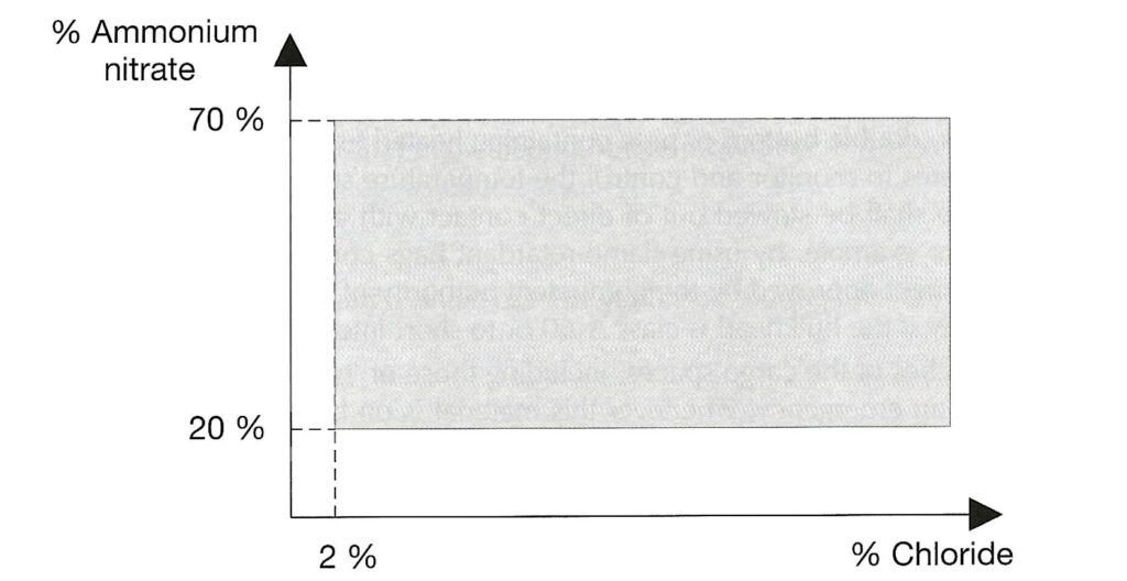
AMMONIUM NITRATE BASED FERTILISER. Note that the designation “non-hazardous” is no longer present. This is a Group C schedule which, together with the MHB schedule below replace the old “non-hazardous” schedule. The Group C schedule says it applies to mixtures which fall within certain limits defined by the amount of ammonium nitrate and the amount of chloride present. To be within the Group C schedule, the material has to fall within the grey shaded area in the graph reproduced below. Note that either the amount of ammonium nitrate is very low or the amount of chloride is very low (or both).
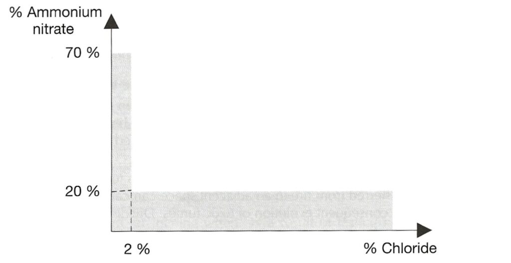
There is a provision in this schedule that materials which fail the trough test are excluded from the schedule. It is a stated hazard that Group C ammonium nitrate based fertiliser will decompose if exposed to heat, but that decomposition is “highly unlikely” to spread through the bulk.
AMMONIUM NITRATE BASED FERTILISER MHB is the final schedule, and this is wholly new. It is categorised as Group B, hazardous only in bulk (MHB) of type “OH” (other hazard). This means a hazard which is not one of the standardised ones. The schedule includes a definition in terms of compositional basis to distinguish it from the Group C material above. The graph is the complement of the one reproduced above – i.e. it covers material with more ammonium nitrate or more chloride or both but not sufficient ammonium nitrate to make the material one of the more hazardous types.
Again, the schedule states that material which fails the trough test is excluded. This MHB schedule only applies to substances which pass the trough test. However, this schedule states that this material has the hazard that an initiated decomposition event can propagate through the bulk.
This new schedule then accommodates ammonium nitrate fertilisers which pass the trough test but do actually possess the hazard the trough test was designed to detect. The schedules appear to have been written in this manner as a work-around for the fact that the trough test does not detect all fertiliser mixtures which can undergo self-sustaining decomposition.
I note that historically, research has shown that self-sustaining decomposition is only a possibility with a mixture which includes ammonium nitrate and chloride (generally NPK fertilisers where the K element is supplied by potassium chloride/muriate of potash). That is the basis behind the graphical composition criteria.
Working backwards, the effect of the new provisions is as follows. Firstly, materials which are compositionally UN1942 or UN2067 remain covered by those schedules. Any other fertiliser material which contains ammonium nitrate and fails the trough test is Class 9 UN2071.
The remaining two schedules apply to any substances which pass the trough test, and which one applies depends on the levels of ammonium nitrate and chloride. The implication of the criteria is that ammonium nitrate fertiliser with below 20% ammonium nitrate or below 2% chloride can be assumed not likely to undergo self-sustaining decomposition and can be consdered Group C. The MHB schedule covers the rest, and presumably would have applied to the CHESHIRE cargo and the PURPLE BEACH cargo had the new schedules been in existence at the time those cargoes were shipped. [Note that I am not party to technical data regarding the cargoes on these two vessels but assume this to be the case.]
How does this new set of schedules benefit the seafarer? Well, the MHB schedule is the one to focus on because it encompasses substances which were prevoiusly categorised as non-hazardous despite being capable of leading to the total loss of a vessel such as CHESHIRE. The big difference is that the seafarers will be aware of the potential risk and will therefore be more likely to detect it early if it happens. The Code outlines a number of precautions to be taken when MHB ammonium nitrate based fertiliser is carried, and some provisions indicating what to do if a decomposition event is detected during the voyage.
Hopefully the new schedules will assist in avoiding these horrific events.
A new Code – Part 1
It has been a while since I wrote here. Things have been madcap busy at Sheard Scientific. There’s just enough time now after digesting another turkey lunch for me to digest the contents of a new edition of the IMSBC Code, which landed on our doormat here at Sheard Scientific this month. I will start with this article by outlining what is in the Code and how it all works. Tomorrow, I will set out what has changed.
This tips the scales at a hefty 2.2kg. Quite a weighty document – the bulky code perhaps!
There is of course a reason for this. When the old BC Code morphed into the first version of the IMSBC Code and became mandatory under SOLAS, it contained schedules for individual bulk cargoes and a mechanism for missing or incorrect schedules to be identified and added. Those processes have been in place now for a number of years, and on each new edition, the Code gets bigger and bigger, and heavier.
The concept was that any cargo carried in bulk (other than grain cargoes, and many don’t properly understad why they are not covered) will have its own schedule. In that schedule will be a listing of the properties and hazards of the material and guidance regarding carriage.
The amendment timetable has been disturbed a little by Covid. The new edition is now available in print, and can be applied on a voluntary basis from 1st January 2023 and becomes fully mandatory on 1st December. This pattern – of publication followed by a period of voluntary applicability and then full force has been the case for previous amendments.
It is important to note that the concept of “voluntary” applicability is voluntary in the sense that the relevant Competent Authority/participating governmental body to IMO can decide that the new Code applies. It is not left to be a voluntary decision by individual shipowners, ship Masters, or indeed cargo shippers.
As the amendments to a document such as the IMSBC Code by definition represent best practice in the industry, it should in my view be in everyone’s interest for the amendments to be adopted as soon as practicable.
It is worth taking a quick look through the material making up the Code as published. Some things are in surprising places – this is to an extent a legacy of a shake-up of organisation as the material which used to be in various locations in the BC Code is mostly still to be found, just not necessarily where you might think it would be.
Sections 1-13 are where procedures, rules and regulations, and definitions are to be found. Material specifically relevant to liquefaction for instance can be found in sections 4, 7, 8, but you might also need to check section 5, which relates to trimming. There really is no substitute to reading through these sections carefully even if just to know what can be found where.
The next part of the Code is the appendices. Unlike most books, the appendices to the IMSBC Code are a fundametal part of the contents. Appendix 1 on its own is nearly 400 pages long, and contains the individual schedules for bulk cargoes, listed alphabetically by Bulk Cargo Shipping Name. These schedules are the part of the Code which a vessel’s Master will spend most time looking through, and this is the part of the Code which enlarges on each amendment as additional schedules are added.
Appendix 2 contains test methods applicable to bulk cargoes. This includes all six tests for Transportable Moisture Limit along with other tests.
Appendix 3 is headed “Properties of solid bulk cargoes” and is a curious mixture of seemingly unconnected but very important sections. One important point to bear in mind is that the contents of this appendix are not legally mandatory under SOLAS whereas some other parts of the Code are.
- Appendix 3 point 1 is a list of non-cohesive cargoes (as contrasted with other cargoes which are considered cohesive) and some provisions which flow out of this property.
- Appendix 3 point 2 is a single paragraph which describes the types of cargoes which might undergo liquefaction or dynamic separation. This paragraph is often quoted in disputes, so I will quote it here.
Many fine-particled cargoes, if possessing a sufficiently high moisture content, are liable to flow. Thus any damp or wet cargo containing a proportion of fine particles should be tested for flow characteristics prior to loading.
IMSBC Code Appendix 3 paragraph 2.1
- Appendix 3 point 3 is a provision which states that where a Competent Authority has to be consulted prior to shipment (i.e. substances not listed in the Code or substances with hazards which differ from that listed in the Code), the corresponding authorities at the loading and discharge port should be consulted. This is to ensure that all potentially involved in the carriage of a substance with chemical hazards are aware and agree with the precautions being taken.
Appendix 4 is the Index. However, it is much more than just an index. As stated above, the list of schedules in Appendix 1 is arranged alphabetically and so acts as its own index to an extent. In Appendix 4, the Index also includes entries which cross-reference to a BCSN. These can be found in lower case entries in the Index whereas entries in capital letters are the BCSNs themselves. As an illustration of how this works, the fourth entry in the Index is ALUMINA HYDRATE, a Group A&B cargo. The capital letters denote that ALUMINA HYDRATE has a schedule under that name in Appendix 1. Lower down on the same page can be found Aluminium hydroxide. As this is in lower case, it isn’t a BCSN and there is no schedule in Appendix 1 for Aluminium hydroxide. However, the entry says “see ALUMINA HYDRATE” and so the reader is thus informed that aluminium hydroxide and alumina hydrate are synonymous from the viewpoint of the entries in the Code. There are many other examples of this type of cross-referencing in the index.
Appendix 5 is similar to an Index but contains BCSNs from the Code in English, French and Spanish.
The rest of the book as published is the Supplement to the Code, and this amounts to a further 150 pages.
The documents making up the Supplement are all also published separately in their own right or as IMO circulars. They cover a wide range of topics, starting with the BLU Code (Code of Practice for the Safe Loading and Unloading of Bulk Cargoes) and ending with an alphabetic list by country of the designated Competent Authorities.
More or less in the middle of the Supplement can be found the document “Recommendations on the safe use of pesticides in ships applicable to the fumigation of cargo holds” which is also published as IMO Circular 1264. This is a vitally important set of guidelines and recommendations which is essential reading for any becoming involved with shipboard fumigation, whether that is carried out in port or when continued in transit. I mentioned this circular earlier this year in the context of a serious incident involving fumigation.
Sugar cargoes – a visit to the Museum of London Docklands
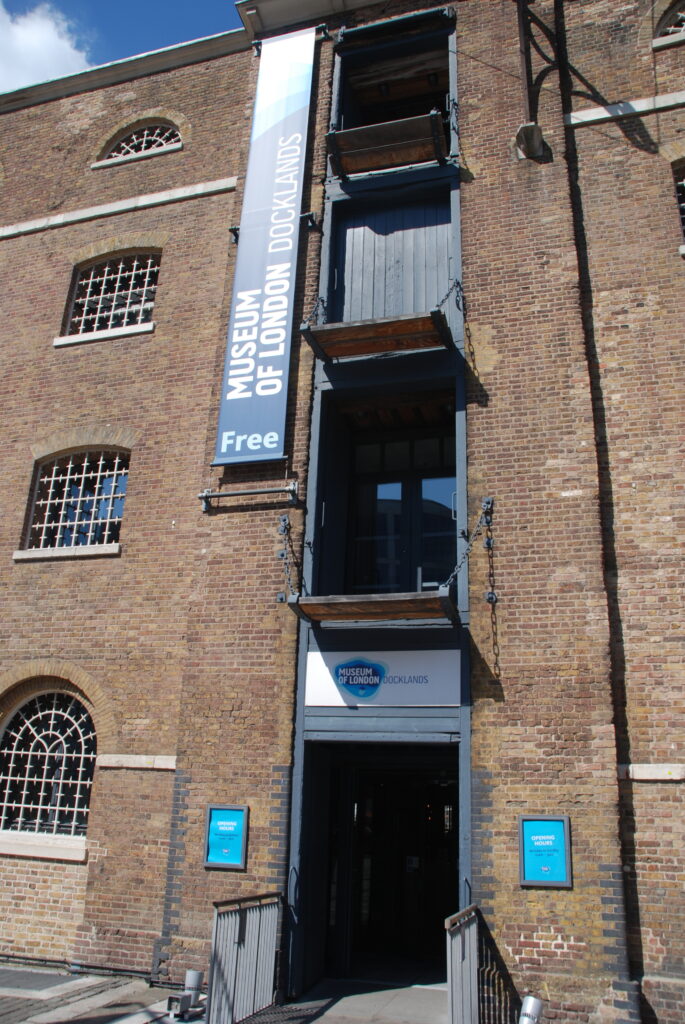
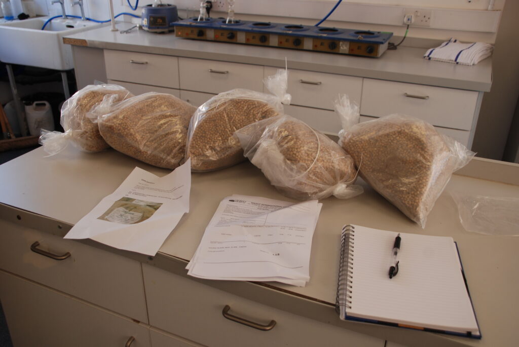
Having been in London to attend an analysis at the GAFTA laboratory Salamon & Seaber, we paid a visit to the Museum of London Docklands, to be found in the shadow of Canary Wharf at West India Quay.
It’s a fascinating museum with mock-ups of the London docks in their heyday, information on equipment and the working practices. There’s also a whole section on the effect of the second world war and the bombing of the docks. Well worth a visit.
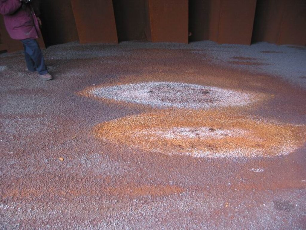
What caught my eye as a cargo scientist was an area on sugar. Much of this focussed on the terrible history of slavery associated with sugar production. This was fascinating and sobering, and certainly told me much I had not previously been aware about regarding that trade. There was also information about the cargo itself and its production, one form of which is still imported into London docklands to be refined. That cargo is shipped in large quantities and will be the topic of this article.
“Sugar” can refer to one of a large range of chemical entities falling under the heading “sugars”, but when it is used to refer to a cargo on a ship, that cargo will be sucrose sugar, which is the substance used to sweeten tea and coffee, and in baking. Sugar crops are grown as sugar cane in the caribbean and elsewhere, and sugar beet in temperate climes. Once the sugar has been extracted from the parent plant, its origin (i.e. whether it came from beet or cane) is less significant than how much and what type of processing or refining it has been subjected to.

If this molecule is broken in the middle, two smaller sugars are produced – the left one is glucose (the fundamental fuel for cellular life) and the right one becomes fructose (the sugar found in fruit). That splitting happens in real life by reaction with water (hydrolysis), and that is a very important process to understand.
Sugar is carried by ships as one of two main types – raw sugar, which is usually carried in bulk, and refined sugar, which is usually to be found in bags. For the purposes of carriage, these behave very differently and require different consideration from the carrying vessel.
Raw (bulk) sugar
This, as the name suggests, is sugar which has received relatively little processing. It is off-white or darker in colour, granular, but doesn’t flow readily. The most important thing to bear in mind when dealing with raw/bulk sugar is that it will be intended to be subjected to refining prior to use. This means that raw sugar is one of the least sensitive cargoes when undergoing carriage at sea.
Even sugar from a hold which is submerged in water will contain substantial value. There are a number of consequences of water ingress into bulk sugar. One of these is simply that the sugar contains water. Thus a tonne of cargo discharged will contain less actual sugar than a tonne of the cargo did when it was shipped. This isn’t a real loss, but it does make it more difficult to keep track of the quantities of cargo being discharged and handled post-incident. I have seen severe incidents, where a hold has become tidal, where some of the sugar/syrup has washed out of the hold. That of course is a real loss, and it then becomes very important to keep track of how much sugar is in the various parcels eventually off-loaded.
The presence of water or excess moisture will also accelerate hydrolysis reactions as mentioned above – some of the sucrose di-saccharide molecules will react with water to produce glucose and fructose molecules. These will be removed in refining, meaning that the amount of refined sugar produced will reduce. This is also a real loss, but it is evaluated in a different way.
I discussed the basic equations of electromagnetism (Maxwell’s equations) a while ago. To explain how damage to bulk sugar is assessed, I need to talk a little about polarised light. The Poynting vector points in the direction the ray of light is travelling, but the electric and magnetic fields which make up the light wave are at right angles to this vector (and to each other). Thus a light bean travelling directly away from you may have electric field directed vertically up/down and magnetic field left/right. Most sources of light are a combination of differently oriented electric and magnetic fields. Plane-polarised light has each of these fields only present in one direction. Polarised light can be created by the light source but it can also be created by polarising or “polaroid” sunglasses. Thus a non-directional light source such as light from the sun outside can be made into polarised light by passing it through a polaroid filter. As this cuts out all light oriented in the perpendicular direction, it reduces the intensity of the light passing through. That’s why polaroid sunglasses help on bright sunny days.
Once you have created polarised light by passing through a polaroid lens, it remains polarised with that orientation until something else happens. If you pass that light through a second polaroid lens, what happens depends on the orientation of the second polaroid. If the two polaroids are lined up, the light will pass straight-on through the second. If they are oriented at 90° to each other, there will be no light at all passing though the second lens. Try it. Hold two polaroid lenses (perhaps two pairs of sunglasses) up to the light and rotate the second pair relative to the first. You will see it go successively light and dark as the lenses line up.
What’s that got to do with sugar? Good question. Sugar solutions have the property that they can rotate the orientation of plane-polarised light. So if you have your two polaroid lenses at 90° and shine a light through (any light), you get no transmission through past the second lens. Put a sugar solution in between the lenses, you suddenly get light transmission again. To get no transmission, you would have to rotate the second polaroid. The angle you would have to do that by is a measure of how much the sugar solution rotated the plane polarised light.
A test carried out with a sample of sugar will make up a solution in a prescribed manner and establish the angle by which that solution rotates plane polarised light. From this is calculated a number called “pol”, which is expressed as a percentage. Pure sucrose has a pol of 100%.
Adding water reduces the pol (but as stated above doesnt actually reduce the amount of sucrose. Hydrolysis of sucrose to form glucose and fructose not only reduces the concentration of sucrose (and thus reduces the pol for that reason) but, because fructose rotates plane polarised light in the other direction to sucrose, hydrolysis actually reduces the pol by more than the amount of sucrose which has been hydrolysed.
Thus, if you have a cargo of bulk sugar, it is very important to sample it properly and representatively, and then measure the moisture content and the %pol. From these figures it is possible to calculate how much damage the sugar has suffered. Usually it isn’t as much as might be imagined from the cargo appearance.
As bulk sugar is hygroscopic, it should be ventilated according to the normal rules of seamanship. Having said that, condensation isn’t going to cause any genuine problems, so it doesn’t really matter what ventilation is applied.
Refined (white) sugar
This is usually carried in bags. There are a number of different grades of refined sugar, and I’m not going to go into the differences here. As a refined product, it is usually intended for direct human consumption. It tends to have a very low moisture content and will readily absorb moisture if exposed to the atmosphere.
Traditionally, the bags are made of woven white polypropylene, and they have a plastic film inner liner, which is stitched to the outer bag structure at each end. The polypropylene provides the mechanical strength and the film liner provides a moisture barrier. The moisture barrier is not a complete one – some moisture can get through the plastic film, and also moisture or even water can penetrate the film where the stitching has made holes in it. But the presence of the liner largely separates the very dry and hygroscopic sugar from the in-hold atmosphere. This means that for practical considerations, the sugar cargo in bagged form is not hygroscopic. Bagged refined sugar should not be ventilated. There are no circumstances in which it would be necessary to ventilate bagged sugar.
Indeed, there are circumstances where applying ventilation to bagged sugar can cause damage. Two mechanisms come to mind. The first is the classic “cargo sweat” situation. If inherently cold bagged sugar is loaded and carried to a warmer climate, and ventilation is applied, that can lead to condensation directly onto the bags and wetting of the bags. The sugar will remain cold throughout even a long voyage, and warm moist external air can cause substantial condensation onto the bags, particularly if the vessel has mechanical (i.e. fan-assisted) ventilation facilities.
The second mechanism is that ventilating with air of different temperature to the bags (warmer or cold) might be said to induce temperature fluctuations which could give rise to caking. As caking is one of the biggest problems experienced with sugar, it is important that nothing is done which might promote that caking.
Folklore suggests that sugar in lined bags can come into contact with splashes of water, but that isn’t recommended. Heavy condensation or wetting as a result of water ingress will have a tendency to penetrate the bags through the stitched ends. If that has happened, a region of syrupy sugar will be found at the end of such a bag when it is cut open. Most of the water will run off the lined bags, with only a small amount gradually seeping in through the stitches. This means that a stow of sugar in bags where there is water ingress from (say) a hatch cover leakage will suffer disproportionate numbers of damaged bags as a consequnce when compared to bags of rice which absorb much more of the water in the first few tiers affected. In way of a leakage, the water will find its way downwards leaving a pyramidal structure of wetted bags. The actual amount of water damaged sugar will be relatively small but that will be distributed amongst many bags.
Problems can also occur if bags are handled roughly, as the film liners can become torn. Likewise, if stevedores use hooks to lift the bags, the film liners will become compromised.
As I have said above however, caking is the most problematic issue with refined sugar, and that does not require damage to be bags or water ingress. Many articles have been written describing caking and what sort of inspections to carry out on caked bags identified after carriage. There are things you can do to investigate – like picking bags up and dropping them, cutting bags open to see whether the caking is present throughout or just the ends, and so on.
Sugar can cake very hard indeed. That is usually associated with the sugar not having been properly conditioned after refining. If sugar is bagged without conditioning, it can be too warm, too moist, or with moisture not equilibrated. These factors tend to give rise to hard caking by means of sugar being deposited in crystalline form between two adjacent granules, binding them together. If that process happens extensively in a bag, it can result in sugar which is wholly moulded to the shape the bag was compressed into in the stow without there being any straightforward means to return the sugar to its original free-flowing nature.
If a vessel is loading sugar which hasn’t been properly conditioned, there isn’t much they can do to prevent or reduce caking. It is a good idea to get an idea of the temperature of bagged sugar at the time of loading – but not using a spear thermometer!
Now we are Six
Absolutely nothing to do with A.A. Milne – sorry!
Iron ore fines
I outlined in last week’s post the three tests which have been a familiar part of the IMSBC Code for many years. In 2009 there were two vessels lost in India carrying iron ore fines – ASIAN FOREST and BLACK ROSE. In addition, there were numerous problems which arose during the loading of other vessels. At the time there was no schedule in the Code for iron ore fines as a Group A cargo. As a consequence, work was carried out resulting in new schedules and a new test. As I noted, the existing three tests came in for some criticism for not giving consistent results across a range of different types of iron ore fines. As a consequence, a new test was developed, which is now a part of Appendix 3 of the Code.
That test was based on the Proctor/Fagerberg test, and is referred to in the Code as the “Modified Proctor/Fagerberg test procedure for iron ore fines”. This test methodology makes it clear that it should only be used to test samples of iron ore fines.
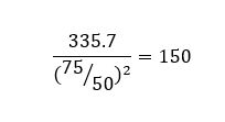
The standard equipment set was used but with a much lighter compaction hammer. This hammer weighs only 150g – less than half the mass of the standard hammer. The size of hammer required for the test was established by reference to work on the conditions experienced in a typical stow of iron ore fines, but it is very light indeed and imparts only small blows on the moulded sample. Even toffee hammers weigh more!
Incidentally, in Proctor’s original work on testing soils, the hammer weighed 2.5kg. Reducing the hammer size to 350g (standard Proctor/Fagerberg, referred to as the “C” hammer) and then 150g (modified P/F, referred to as the “D” hammer) provides substantially less energy input.
Unlike the standard Proctor Fagerberg test, the modified test for use with iron ore fines defines TML as the moisture required to produce 80% of saturation level. The justification for moving the critical point from 70% to 80% is touched upon in the wording of the test methodology in the Code. It says.
Optimum moisture content (OMC) is the moisture content corresponding to the maximum compaction (maximum dry density) under the specified compaction condition. … This test procedure was developed based on the finding that the degree of saturation corresponding to OMC of iron ore fines was 90 to 95%, while such degree of saturation of mineral concentrates was 70% to 75%.
IMSBC Code 2020 Edition, Appendix 3.
The concept of OMC is an important one. Imagine a sample with no water at all. Compaction using the hammer will result in a density which is governed by the intrinsic density of the solid material in the sample together with how well it packs into the mould (i.e. how much air remains after compaction). When water is added, initially the water will assist in lubricating particle to particle contact and will fill some of the voids – thus the density will increase because there is water in the gaps rather than air. Eventually, further additions of water will result in some free water within the sample mould because the voids are as filled as they can be. Because the density of water (1 kg/m3) is lower than the particle density of the ore being tested, adding further water serves to reduce the overall density. A mathematician would refer to this as a “turning point” in density, and the highest density happens at a moisture content known as OMC. OMC will depend on the compaction conditions – i.e. the weight of the hammer and to a lesser extent the shape and size of the mould.
Hence reasoning behind having a higher criterion for TML in iron ore fines. As the Code says, the iron ore fines samples studied had a higher saturation at OMC than was found when studing mineral concentrates using the Proctor/Fagerberg test. The aim is to set a TML which maintains a good safety margin (recall that for the flow table test and penetration test, TML is generally set at 90% of Flow Moisture Point). The reported fact that iron ore fines can typically attain a higher saturation than do concentrates means that the TML can be safely set to a slightly higher saturation level (80% rather than 70%). Well, that’s the theory.
As noted above, the modified Proctor/Fagerberg test for iron ore fines is only applicable to that cargo. This was the first time a TML test had been written into the IMSBC Code which related only to a specific cargo. Note that there is no prohibition on using any of the the original three tests on iron ore fines. The modified Proctor/Fagerberg test for iron ore fines is likely to give higher TML figures than would using any of the other three standard tests. It is odd that one of the driving forces beind the development of the modified test was that the existing three tests did not give consistent results. We now have a situation where a sample of iron ore fines can be tested by any of four methods, and these do not give similar results to each other.
Coal
The next method found in the Code is a modified Proctor/Fagerberg specifically for coal.
It is curious that the standard Proctor/Fagerberg method in the IMSBC Code contains the following statement
This method should not be used for coal or other porous materials.
IMBC Code 2020 Edition, Appendix 3, methodology for standard Proctor/Fagerberg
The way this provision is written is suggestive that the underlying reason the standard Proctor/Fagerberg method is unsuitable for coal samples is because coal is porous.
The modified method for coals uses a similar overall procedure to the standard Proctor method but the vessel has a larger diameter. The test method calls for a “hammer equivalent to the Proctor/Fagerberg D energy hammer” – more on this curiously worded requirement below. Critical moisture is set at 70% saturation, which is the level used in the standard test. If 70% of saturation cannot be attained in the test, the conclusion is that the cargo is not liable to liquefy. It is not clear to me how this addresses the implied difficulty in testing coal/porous materials implied by the wording of the standard method.
As noted above, the coal test method calls for a hammer equivalent to the D type energy hammer. That is the hammer developed for use with the iron ore fines test, which weighs 150g and has a foot diameter of 50mm. However, the image of the equipment for the coal test shows a different hammer. This has weight 337.5g (nearly as much as the standard C type hammer of 350g). However, the diameter of the foot is 75mm whereas the size of the standard D hammer is 50mm across. Thus the hammer shown for the coal method is heavier than the iron ore fines hammer but has a larger foot. It is equivalent because
The most striking novel feature of the coal Proctor method is a procedure to create a reconstituted working sample where the coal contains particle sizes in excess of 25mm. Many commonly traded coal cargoes are sized up to 50mm, and so many real world coal cargoes will require the reconstitution procedure to be applied. The reconstitution process involves removing “oversize” (i.e. over 25mm in size) and then adding back calculated proportions of smaller particles from the working sample to replace the removed oversize fraction.
I mentioned in my earlier post on testing that a work-around to deal with oversize was in widespread use for nickel ore. The reconstitution process for coal samples is a part of the new modified Proctor/Fagerberg test for coals and is the first approved means of testing samples with particles larger than 25mm.
Many types of coal are not capable of liquefying and are thus not Group A cargoes. Very helpfully the new test contains criteria for determining if a coal is liable to liquefy.
I note that the new modified method for coal states that it requires a minimum of 170kg for a test to be carried out.
There are now three tests which can in theory be used for coal – the flow table test, the penetration test and the modified Proctor/Fagerberg for coal. The new coal test contains a number of elements which are not present in the flow test or penetration test – i.e. the ability to modify samples to allow for the presence of much larger particles and the existence of a diagnostic check in the test to determine whether a given coal is Group A or not.
Bauxite
The final method is specific to bauxite. The existence of this test came about as a consequence of the BULK JUPITER sinking and the work carried out which established and characterised dynamic separation as relevant to bauxite.
This modified Proctor/Fagerberg test uses the same larger diameter mould called for to test coal. The hammer is the lighter “D” hammer per the iron ore fines method in its 150g diameter 50mm form.
The bauxite method also contains a method for making a reconstituted working sample by removing oversize and substituting smaller material according to a formula/recipe.
The critical saturation level is set at 70% for some bauxites and at 80% for others. The decision between 70 and 80% saturation as the critical point is made by reference to the optimum moisture content – i.e. the highest saturation attained. This choice has at its technical base the same fundamental issue which is given as the rationale for applying a critical level of 80% in the modified test for iron ore fines as discussed above.
As I have discussed in an earlier article, bauxite is said not to undergo liquefaction in the normal sense, but rather to exhibit dynamic separation when overmoist. Dynamic separation is a different failure mechanism to liquefaction. However, the test introduced to ensure safe carriage and a suitable TML is largely the same as that applicable to iron ore fines.
This test is relatively new, and I have personally only seen it in action once. That particular bauxite formed large clay-like lumps with the addition of water and the 150g hammer was not capable of packing the ore into the Proctor mould except at very low moisture contents. Some bauxite types may be more suited to testing using other methods.
Concluding remarks
The recent proliferation of new cargo-specific versions of the Proctor/Fagerberg, together with the three more established standard methods presents a somewhat bewildering picture. Shippers involved in trades for coal, bauxite or iron ore fines will have the option of instructing a laboratory to carry out the cargo-specific test or one of the standard ones. Different commodities may involve the reconstitution procedures to accommodate substantial oversize. For commodities where no “new” cargo-specific test exists, the laboratory will have no established reconstitution procedure and will have to deal with oversize particles in an ad-hoc manner.
Clearly this is unsatisfactory. If reconstitution works for coal or for bauxite, it would be expected that a similar procedure might work for iron ore fines with oversize, or indeed nickel ore which tends to have oversize.
If it is acceptable to relax the Proctor/Fagerberg critical saturation percentage to 80% for iron ore fines and some bauxites, why is it not acceptable to apply 80% to any cargo which has an optimum moisture content (OMC) of over 90%?
If the studies showed that the new tests provide an appropriate TML for bauxite, iron ore fines and coal, where does that leave the “standard” methods in relation to these commodities? My understanding is that the modified Proctor tests introduced recently for these specific cargoes in a number of instances produce higher results for TML (i.e. the cargo can be shipped with higher moisture content). Perhaps the extra safety margin associated with the older tests was unneccesary.
It is possible to attempt to use the new tests for coal and bauxite and be directed by the test protocol to a conclusion that the subject cargo is not Group A. There are criteria in the schedules for iron ore fines, manganese ore fines and bauxite which set out technical parameters for what constitutes a Group A cargo of that mineral. There are no test procedures or criteria available for other materials to determine whether a given substance is Group A or not.
A number of materials mined and subject to relatively little processing contain a variety of minerals. For instance, an ore may contain nickel and also substantial amounts of iron. If an ore from Malaysia contains aluminium and also iron in oxide form, is it bauxite, or is it iron ore?
In my opinion, the proliferaton of multiple cargo-specific tests makes life very much more complicated for those involved and is not a helpful development. I believe it would have been preferable to revise the test methods in the Code to have either a single available test or a number of tests with the selection prescribed by the Code, rather than a “choice”. As always, however, we recommend adhering to the provisions of the Code wherever possible.
Testing, testing, 1, 2, 3
I wrote last week about liquefaction generally and tried to set the scene. Fundamental to safe carriage in the IMSBC Code is the concept of Transportable Moisture Limit (TML). It has been suggested that a single figure for a cargo does not properly reflect all possible behaviours, but in my experience the safety margin built into the Code is sufficient that if you apply the TML concept properly, the cargoes will carry without significant incident. Indeed, the idea of a TML has gained such traction recently in the maritime industry that I sometimes see figures for “TML” on declarations for agricultural cargoes which aren’t Group A at all – it is being erroneously used to indicate the maximum safe moisture level for avoiding cargo deterioration on board.
Returning to Group A cargoes, Section 8 of the Code tells you that there are test methods for determining TML, and the standard/recommended ones are to be found in Appendix 3 to the Code.
Unfortunately, Appendix 3 is where testing starts to get complicated. There are now no fewer than six different methods listed in the appendix. Three of these are variations on the Proctor Fagerberg test modified to be suitable for specific commodities and are relatively new additions to the Code.
Until recently, there were three methods listed in the Code, and those three will be the subject of this article. It has always been within the power of the various member Competent Authorities to approve alternative test methods, but as far as I am aware this has never been commonly encountered if at all. Furthermore, until relatively recently, the only method widely available internationally at commercial labs was the Flow Table Test.
The concept of TML was developed from another parameter, the Flow Moisture Point (FMP), and the original research into safe moisture levels and cargo testing was carried out on metal sulphide concentrates. Concentrates such as lead, zinc and copper have been shipped for many years and all tend to be Group A cargoes.
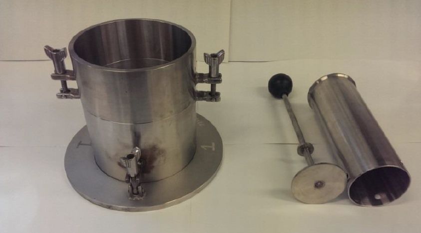
Flow Table
The flow table test measures FMP, which is defined as the moisture content at which a commodity starts to exhibit flow properties. The test involves inputting energy in a defined manner into the sample and monitoring the behaviour of the sample under those conditions.
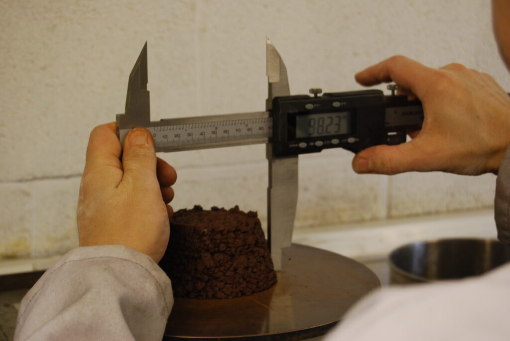
Flow is defined for the flow table test when the cone of sample on the table spreads by a certain amount or slumps. If the sample doesn’t exhibit flow, water is added and the test repeated until it does. By this procedure, the flow moisture point is established by actually determining the moisture content of samples which have shown flow properties during the test along with those which do not.
One potential difficulty with the flow table test is that the methodology requires the operator to determine when a sample is in a flow state by observations during the test itself. The Code does not define exactly how, although there are descriptions of what to do.
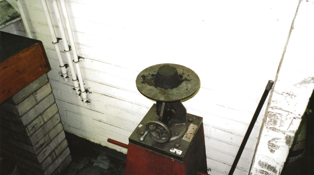
Each test run involves a sample being loaded into the mould in a prescribed way. A spring-loaded device known as a tamper is used to squash the sample into the mould and provide a degree of compression/consolidation to start with. One problem with the flow table test which has largely now been solved is that the necessary calibrated spring-loaded tamper wasn’t available commercially.
Following removal of the metal mould shape, the resulting cone is measured prior to operating the table.
The table is then operated (up to) 50 times. Each turn of the handle lifts the table and allows it to drop 12.5mm. The method calls for the 50 drops to take two minutes.
After the table has been operated 50 times, the resulting material on the table is examined and measured. The IMSBC Code says measurements of the diameter are a useful diagnostic, and refers to a cone expansion of 3mm as being significant. Different laboratories have used this information in different ways. I can’t go into too much detail in this article but if full documentation of the test conditions is available from the laboratory, an expert can see how the stated result was obtained and what criteria were used.
The flow table is relatively inexpensive to buy, but it is important to ensure that a table meets the required design specification.
There are limitations associated with the flow table test. One is a consequence of the physical size of the mould into which the sample is placed on the table and relates to the maximum particle size.
The flow table is generally suitable for mineral concentrates or other fine material with a maximum grain size of 1 mm. It may also be applicable to materials with a maximum grain size up to 7 mm. It will not be suitable for materials coarser than this …
IMSBC Code Appendix 3
Widespread use of the flow table test for nickel ores having a proportion of much larger particles present has now been in place for a number of years, but the “fix” used has never been approved by IMO.
This fix works by considering nickel ore to be an assembly of larger particles embedded in a continuum made up of the more fine material. The flow table test criteria of 7mm is a workable limit for many nickel ore cargoes – removing the material above this size results in a testable working sample. The assumption made is that the liquefaction of the material as a whole (with the oversize) is solely governed by the behaviour of the sub-7mm fraction. The oversize is present in the cargo but is “along for the ride” without participating in the liquefaction. There is a further assumption which is that the moisture associated with the larger particles remains with them when sieved out, leaving the moisture associated with the finer material. Thus if flow table testing is carried out on the 7mm fraction alone, that provides a TML relevant to sieved samples. Provided the average moisture content is also tested on a sieved sample, the effect will be to ensure that the moisture level in the sub-7mm part of the cargo as a whole is below its TML, and hence the cargo can be assumed to be safe.
The obvious problem with this approach is that the moisture content of a sieved sample will tend to be different to the cargo as a whole. Most cargoes are bought and sold on terms which include specifying the cargo moisture levels. That isn’t for safety reasons but rather to act as a control for how much water is being bought rather than (here) nickel-bearing ore. Thus the moisture content entered onto the cargo declaration is not the same as the one used in the cargo sales contract. It is sometimes difficult to establish whether this has been done correctly.
Penetration Test
The penetration test was developed in Japan as an alternative to the flow table test, but it has certain similarities. This test is also repeated with additions of water until the sample exhibits flow properties. For this test, the energy input into the sample is in the form of a vertically oscillating platform onto which the sample is placed in a vessel. These vessels are much larger than the conical moulds used for the flow table test, and hence the penetration test can accept much larger particles.
The penetration test is generally suitable for mineral concentrates, similar materials and coals up to a top size of 25 mm.
IMSBC Code Appendix 3
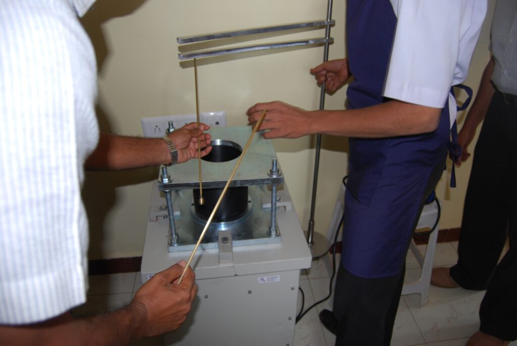
The ability to accept samples containing much larger particles is one advantage of the penetration test. Another is that the definition of a flow state is given in terms of the distance penetrated by brass weights into and below the sample surface during the six minutes the vibrating table is run for on each test run. No subjective observation is required. The rate and amplitude of oscillation of the table are specified in the Code. In the video below a sample of iron ore fines can be seen to enter a flow state – signified by the brass weight penetrating the sample surface. Note that the video has been shortened from the original six minutes.
The flow table test and the penetration test have one fundamental thing in common. During the testing itself, each test run involves taking a working sample and subjecting it to the input of energy. This is meant to simulate the vibrations and motion on a ship, which is when liquefaction might take place. Water is added and the test runs repeated until a flow state is achieved, and thus the flow table and penetration test both create a flow state which the operator will see. In the flow table test, the sample will slump and expand during the test. On the penetration test rig, the metal bit will sink into the cargo sample, and other changes in the sample will be seen – perhaps water will come to the surface or the surface will become smooth.
Equally, if the sample is received in a state in which a flow state occurs on the first test, the operative will know immediately that the cargo as sampled will not be considered suitable for carriage.
The Code defines TML as 90% of the FMP for most materials. That 10% is a safety factor.
Proctor/Fagerberg Test
The third of the three long-standing tests is the Proctor/Fagerberg test. Until relatively recently this was not in widespread use in shipping, but it has always had its fans. This test works on a different principle to the flow table and penetration test. Here, the test runs involve packing the material of the cargo sample into a mould using a hammer. The weight of that hammer is specified by the method as 350g. The different test runs are not designed to result in liquefaction, and indeed no visual observations are required.
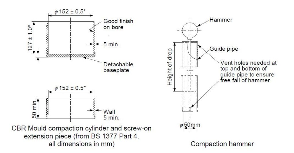
Liquefaction happens when the balance between solid particles, interstitial air and interstitial water is such that rearrangement of the assembly of particles when exposed to energy/vibration results in the interstitial water mediating particle to particle contact. The pressure of that water then supports the material above rather than particle to particle contact. This process was introduced with an illustrating diagram in my last article on liquefaction.
Proctor/Fagerberg replicates that compaction and rearrangement process using the hammer blows. As the density changes with increasing water, the test observations can be used to produce a curve from which the transportable moisture limit (TML) can be obtained.
The Proctor test does not produce an FMP and no observations of the cargo in a flow state will be possible during a test. The calculations required to process the raw data obtained during a test run, in order to plot a meaningful graph and establish a figure for the TML, are somewhat complex, and are a possible source of errors during testing. TML in this test is defined in terms of the moisture required to produce 70% saturation in the sample under compaction. Without the visual observations from the test itself there is no “sanity check” on the result obtained. That is one disadvantage of the Proctor/Fagerberg test.
The IMSBC Code sets out the calculations and invites the tester to plot the following graph.
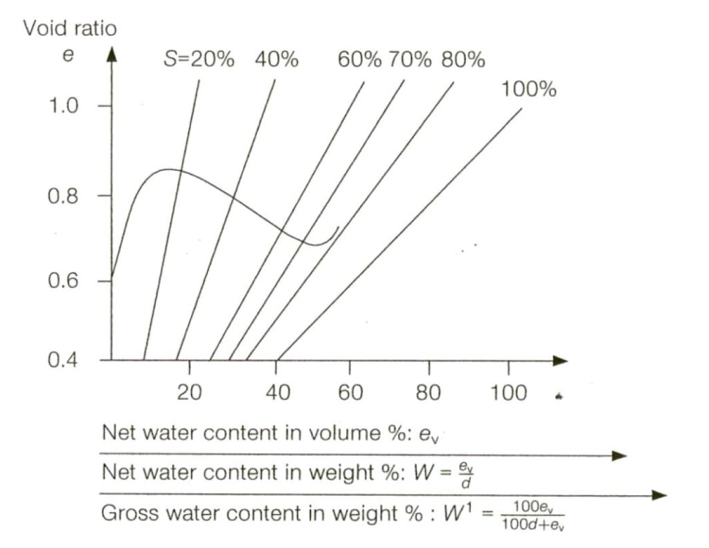
Fortunately the same data can be plotted in a (slightly) more intuitive way, as follows.
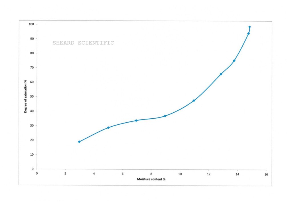
In this graph, the moisture content is plotted vs the degree of saturation that produces in the interstitial void space after compaction using the hammer.
Another disadvantage is again tolerance for large particles. The wording of the standard Proctor/Fagerberg method in the IMSBC Code indicates that it is suitable for materials with maximum particle size up to 5mm. The method goes on to imply that the method can be extended to work on substances having larger particles present but this needs to be investigated prior to deployment. Furthermore, the method states it is not suitable for coal cargoes.
For many years, those three methods were the only ones included in the IMSBC Code. For many mineral concentrates, the three methods would tend to give reliably similar results. Indeed, that was no coincidence. The parameters and TML criteria for the penetration test and the Proctor/Fagerberg test were in both cases selected in order to give similar results to the flow table test on some commonly-encountered mineral concentrate cargoes.
The problems started to become highlighted with the large-scale shipment of (first) nickel ore and then iron ore fines as Group A cargoes. Unlike mineral concentrates generally, these are not heavily processed commodities, and their behaviour when tested is not comparable with concentrate cargoes.
Nickel ore presents a number of challenges to a flow test. I have already mentioned the work-around in widespread use for large particles. Whlist this works, I don’t consider it particularly satisfactory. Unlike concentrates, nickel ore does not have a clearly defined transition from a dry state to a fluid liquefied state – you tend to find, if using the flow table test, that the cone expansion increases gradually over a wide range of moisture contents. Vagueness in the definition of flow state has resulted in large discrepancies in results between different laboratories when testing this material.
Iron ore fines entered the public gaze (the shipping public gaze, at least) a few years later. Iron ore fines cargoes of differnet origins can behave very differently when under test, and some cargoes also present the “oversize” problem but to a lesser degree than nickel ores.
There was considerable debate at IMO level regarding how to test iron ore fines for TML. The existing tests received some criticism for not giving consistent results for this commodity. As a result, when the IMSBC Code was revised to incorporate a schedule specific for iron ore fines, a new test was included at the same time. This test methodology was first published by IMO in late 2013 but was not fully incorporated as a mandatory part of the IMSBC Code until 2017.
Liquefaction – some basics
By now, most of those involved in shipping bulk cargoes know that some commodities can undergo liquefaction. Quite what that means is less well known, but it is very well publicised that it can result in ships sinking. Articles regularly appear setting out how many ships have been lost and the number of people who have lost their lives when their vessels have got into difficulties during carriage.
There is much less information available on the “nearly” events, or even the “we worked hard to avoid” events. I have personally been involved in a substantial number of both of these. Timely advice and/or intervention can save ships and lives. I’m pleased to be able to say that no vessel I have been involved with has subsequently been lost. Suffice it to say that the cost to the industry of problems arising from liquefaction generally is very high.
IMO categorises bulk cargoes which can liquefy as being in cargo Group A.
To comply with the regulations, the moisture content of a Group A cargo needs to be below the transportable moisture limit (TML).
Concentrates or other cargoes which may liquefy shall only be accepted for loading when the actual moisture content of the cargo is less than its TML
IMSBC Code 2020 Edition paragraph 7.3.1.1
What is TML and how is it measured? In a classic example of circular definition, the Code tells you that TML is
Transportable moisture limit (TML) of a cargo which may liquefy means the maximum moisture content of the cargo which is considered safe for carriage in ships …
IMSBC Code 2020 Edition section 1.7
A later post will discuss the tests, as these and how they work is a whole topic in itself.
Liquefaction is a bulk property. One common misconception is that liquefaction involves cargoes becoming a liquid, and indeed the IMSBC Code uses this word to describe a flow state. Many liquefied cargoes however do not behave like liquids. “Fluid behaviour” is perhaps a better term to use.
As a physicist, I will introduce the concept of a phase change, as I believe the analogy is helpful. To a physicist, a change of phase involves a material changing from a state in which it has certain properties to a state where it behaves differently. An obvious example is melting a solid such as ice. Whilst the ice is frozen, its behaviour is like other solids. Melted, it becomes water which can be poured, sloshed, and so on but it is chemically still H2O. The phase change we refer to as melting involves the input of energy. So does liquefaction. A solid bulk Group A cargo can may enter a fluid state if conditions are within certain limits and with the input of energy.
A very widely viewed video shows a wheelbarrow full of soil undergoing liquefaction when energy in the form of vibration over a set of cobblestones is input.
Back in 2009, the year ASIAN FOREST and BLACK ROSE sank in India, I created this diagram.
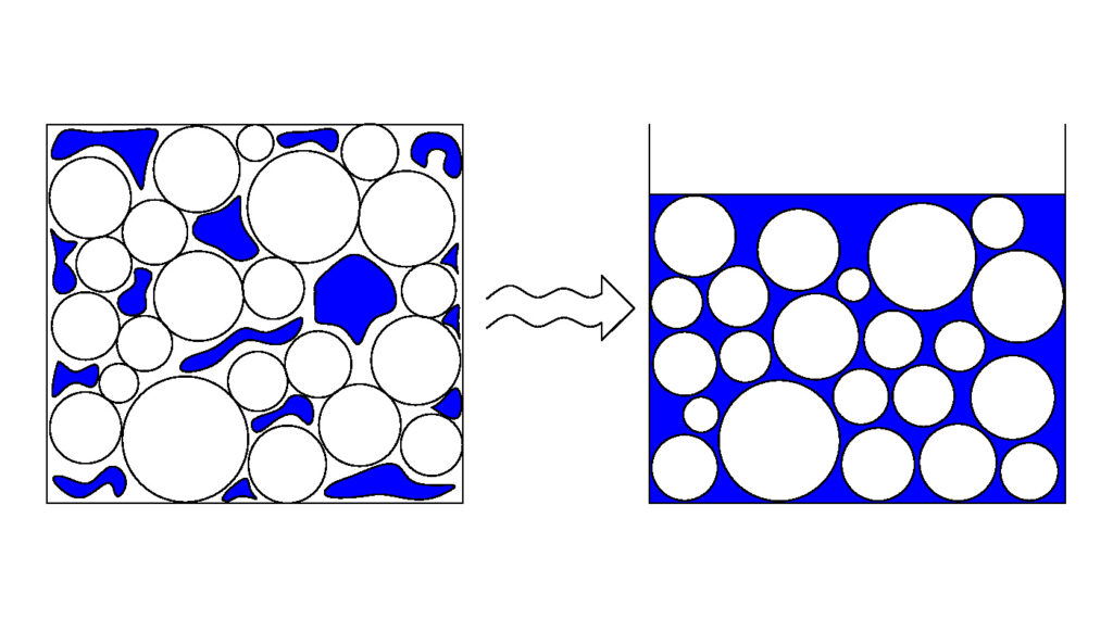
Facsimiles of this illustration exist, even variants where the particles are not circles/spheres. All the attempts to “improve” on my illustration/concept focus on aspects of it which didn’t really need to be updated/modified.
In this example, the assembly of particles is shown to be a collection of spheres (circles in cross-section). That wasn’t chosen because it matches the particles in a cargo of iron ore or nickel ore, but rather because it allows the phenomenon I am illustrating to be clearly seen. The diagram shows a phase change. On the left, the solid particles are loosely packed. There are lots of spaces between them. In those spaces can be found the moisture associated with the cargo (the blue areas). The particles are in contact with each other and the water (blue) is simply present. It doesn’t do anything.
Follow the wavy arrow to the right hand side; there to represent the input of energy in the form of vibration during a sea passage. In the right hand image, you will find exactly the same circles/spheres. Here however the whole assembly occupies a smaller volume than did the left hand image. Thus the input of energy has resulted in consolidation of the cargo into a smaller volume. Further, the image shows blue water throughout the interstitial spaces.
The point the image is illustrating is that the sequence of events involves consolidation/compaction as a consequence of the input of energy. The same volume of solid particles is now associated with less interstitial volume and, if there is enough moisture present, that might result in the water filling the voids on the right hand side when it did not on the left. Liquefaction. The particles on the right are separated by water and it is the water which governs the bulk properties. Pore water pressure is the name given to the pressure associated with the water in the spaces, and in a liquefied stow it is the pore water pressure which supports the cargo above. Water, being a liquid, is nearly incompressible – the volume of water stays the same at all times, it is the volume of the interstitial pores which changes.
The Proctor/Fagerberg test works on this principle – the test is designed to measure the amount of water expressed as a volume percentage of the available space (void/interstitial). Thus the image on the right of my diagram would be 100% saturated in Proctor Fagerberg terms. The energy input in the Proctor test comes from a slide hammer pounding the surface of the sample. I will write about the tests and how they work in a later article.
Many of the provisions in the IMSBC Code (or BC Code as it was a number of years ago) arise from studies carried out on samples of metal concentrates. It is worth remembering this when consulting the Code even today. Concentrates are a semi-manufactured intermediate product and tend to be very consistent in terms of particle sizing. The provisions in the Code allow for TML certification to be up to six months prior to the voyage. These make sense if we are dealing with a cargo of concentrates from a process which churns out parcels of that commodity which are very much the same in terms of flow properties from month to month, even year to year. The same provision makes no sense whatsoever when dealing with shipment of nickel ore or iron ore fines; these receive little processing prior to shipment and the flow properties depend on the geological conditions in the mine.
There are a number of phenomena reported regularly when vessels are affected by liquefaction. As I have said above, the cargoes tend not to behave like liquids, but rather very dense fluids. The stow may flatten out – an untrimmed/peaked stow may turn into a wholly flat surface. There may be water expressed to the surface of the stow. Look at my diagram above – on the right hand image there wasn’t enough room for the inherent moisture and some of it ended up on top of the cargo. That water is simply a liquid and will be free to form a free surface. A free surface of water will affect the stabilty of the vessel but often the amount of water actually on the surface isn’t large, even though it may look spectacular when in motion.
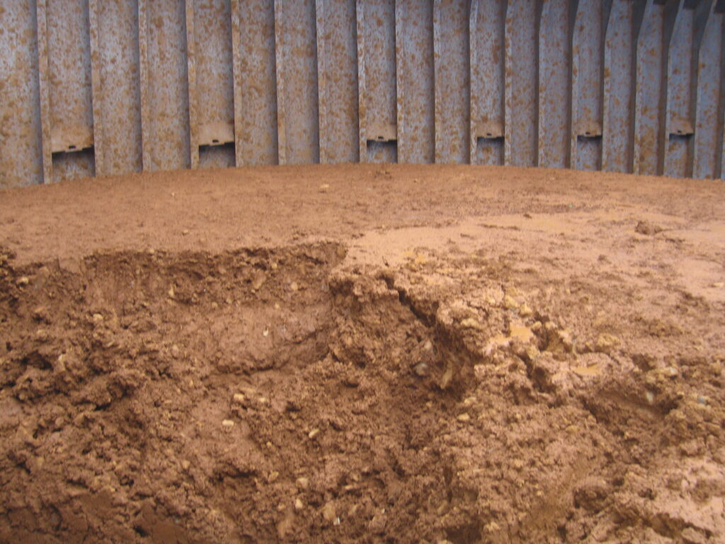
When many cargoes liquefy, the whole stow, or large parts of it, can become mobile. That is a result of the particle to particle contact being prevented by the interstitial water. There are often reports of the vessel taking on a list. This tends not to be an angle of loll, but rather a result of the cargo moving. What can happen is that when the cargo becomes mobile when in a fluid state, it moves to one side with the natural roll of the vessel. It then doesn’t return to centre when the vessel rolls back. Gradually, over a number of roll periods, the cargo takes up position biased towards one side of the hold, resulting in the list. This is of course very dangerous as eventually that list may become large enough for down-flooding with sea water to occur. This is one example of liquefied cargoes not behaving as liquids as it is the asymmetric behaviour of the cargo which results in the list developing.
The case of bauxite as highlighted by the tragic loss of the BULK JUPITER and the lives of 18 of her crew members is interesting. Work followed which resulted in new provisions in the IMSBC Code for Group A bauxite cargoes. It has been strongly argued that bauxite does not undergo liquefaction, and a new term “dynamic separation” has been coined to describe its behaviour. This BIMCO article has a clear description of the difference between dynamic separation and liquefaction. In dynamic separation, the cargo splits into two phases. A lower phase containing the cargo solids is initially immobile despite being saturated with water. It is not in a liquefied state. There is however a volume of free water expressed to the surface (which may be a slurry containing some very fine particles of solid cargo). That water phase is mobile and the risk to the ship’s stability comes from the free surface effect of the water. Only when the vessel’s stability has been compromised by the free surface effect to produce a substantial list might the lower solid phase move.
The new bauxite fines schedule has an interesting provision.
An atypical motion of the ship (wobbling) may also be indicative of cargo instability and the master shall consider appropriate action.
IMSBC Code 2020 Edition
I have heard presentations from members of the bauxite working group where this “wobble” was stressed as one of the clear “red flag” moments a vessel should be watching out for when carrying bauxite fines. A video is often shown which was produced by AMSA to illustrate the behaviour of vessels encountering dynamic separation. I would encourage the reader to watch it carefully.
It is important to note that the video does not show anything liquefying. The motion seen by the model in the video is governed by its buoyancy and the motion of the steel balls in the tracks. Those tracks are shaped to produce a harmonic motion rather like a pendulum. Having two or more balls on the tracks at the same time produces a form of coupled motion. Coupled harmonic oscillators can exhibit extremely unpredictable behaviour. The well-known Rotts Pendulum is an example – this couples two pendulum rods with different lengths and weights. The resulting behaviour can swap back and forth between wobbles and seemingly random modes.
The AMSA video is simply showing coupled harmonic oscillators on a floating system. As an illustration of the consequences of dynamic separation this is appropriate because it is a free fluid phase (the expressed water) which is compromising the stability. This is not the same mechanism which gives rise to the asymmetric behaviour I have described above for cargoes undergoing liquefaction.
For a vessel at a port loading a cargo, the distinction between liquefaction and dynamic separation isn’t obviously significant. Both are behaviours exhibited by Group A cargoes. Both require a TML to be certified and require the moisture content of the cargo to be below the TML for safe carriage. Many natural unprocessed ores contain a mixture of different minerals. Thus the distinction between nickel ore, iron ore and bauxite may depend more on the intended processing and use than the actual make-up of the ore itself.
Vessels carrying Group A cargoes have successfully reached discharge port with mobile cargo in one or more holds. It is however a huge risk. Similarly, carriage of cargo which is overmoist does not necessarily result in either liquefaction or indeed in the vessel getting into difficulties.
The reverse however is clear. To the best of my knowledge, no vessel has loaded cargo which meets the criteria of the IMSBC Code (i.e. with average moisture properly below a reliably tested TML, properly trimmed) and has subsequently had difficulties with cargo liquefaction unless there has been actual water ingress into the holds.
The message then remains the same as it always has. If you wish to carry a Group A cargo safely (and you should), the IMSBC Code should be followed. That means proper sampling being carried out prior to loading, and those samples being reliably tested for moisture and a TML established by a laboratory properly equipped and experienced in carrying out the tests in question. In my opinon there is no substitute for this which can guarantee the same degree of safety.
Mind the Gas
Fumigation of ships and cargoes has for many years been a source of problems to ship and cargo owners. Recently the UK MAIB issued a preliminary report into a serious incident on the vessel THORCO ANGELA, which happened in Liverpool in October 2021.
Insects are a fact of life. The Royal Entomological Society estimates that there are around 1.4 billion insects per each human alive on earth. The total mass of insects on earth is, they estimate, around 70 times the mass of all of the humans.
Hardly surprising then that agricultural cargoes (grains, oilseeds, animal feeds, etc) are at risk of becoming infested. Nobody wants that, and to avoid infestation cargoes must be treated every few months.
Insecticides can be sprayed onto a surface or cargo (“contact insecticides”) or can be applied as a gas (fumigants). Treating a large bulk with contact insecticide would require it to be sprayed (for instance) onto cargo on a conveyor. Using a fumigant is often more convenient as the gas can penetrate a large bulk.
The disadvantage is that it takes time for fumigant gas to diffuse throughout a large bulk. If in that time the gas starts to leak out, that’s bad for two reasons. Firstly, the fumigation may not be sufficiently effective (because the gas wasn’t present throughout the stow for long enough). Secondly, and much more important for safety reasons, if the gas isn’t staying the holds, it is going somewhere else. Fumigants are used because they kill insects. They can also kill humans or at the very least make them very ill indeed.
Most fumigation on ships these days uses a fumigant gas known as phosphine, chemically PH3. With very few exceptions this is deployed on ships by introducing solid preparations (tablets or pellets etc) into the hold. These solid materials contain aluminium or magnesium phosphide. These chemicals slowly react with atmospheric moisture in the hold and release the phosphine gas itself.
Phosphine is very dangerous. The recommended limit for spaces occupied by humans (NIOSH time weighted average) is 0.3ppm. But it isn’t just the toxicity. Phosphine is highly flammable in air, and in the real world, impurities commonly found in it can make it spontaneously explosive. Hatch covers can and have been blown into the air by phosphine explosions. The solid materials themselves can cause fires if they become wetted.
Fumigation on ships is, for these reasons, subject to IMO rules, recommendations and regulations. The IMO publication “Recommendations on the Safe Use of Pesticides on Ships Applicable to the Fumigation of Cargo Holds” has quite an unwieldy title, but contains guidance which should always be followed to ensure safety of life and vessel. This publication can be found as IMO Circular 1264, but it is also bundled as part of the IMSBC Code.
One part of the safety requirements is appropriate signage to indicate when fumigants are in use.
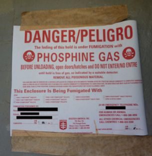
Standard shipboard gas meters are not designed to detect phosphine gas (although they have a sensor which may be referred to as a “toxic gas” sensor, they won’t help in keeping personnel safe). Specialist electronic meters exist, but they are quite expensive and no use for other tasks. Inexpensive glass detector tubes (made by Draeger or Gastec or similar) can be used but each tube can only be used once so you would get through a lot of such tubes in any particular practical deployment.
Lots of articles have set out the provisions to be found in IMO Circular 1264. I’m not going to do that here but I am going to discuss a point which came to the fore during the lockdowns applied as part of the worldwide response to the Coronavirus pandemic.
In the Circular, the following paragraph can be found.
Since fumigant gases are poisonous to humans and require special equipment and skills in application, they should be used by specialists and not by the ship’s crew.
IMO Circ. 1264. Para 3.1.2.2
Recommendations on the Safe Use of Pesticides on Ships Applicable to the Fumigation of Cargo Holds.
This provision is very clearly worded. The pandemic however caused all sorts of problems with many aspects of world trade. One particular trade customarily posted a trained fumigation operative to sail with a vessel as a supercargo. One of his duties was to monitor gas levels in the holds and add more solid phosphide preparation into the holds to “top up” the gas levels. I presume (or hope!) he would also carry out checks to establish where the gas was going, and to ensure that wasn’t going to cause problems.
With the Covid pandemic, this was no longer allowed. Getting personnel on and off ships became virtually impossible in many instances, and so a supercargo riding with the vessel was no longer viable.
The shipping world is full of “make do and adapt” attitudes – admirably so in many instances, but not here in my opinion. Initially, crews were supplied with the solid materials and asked to top up when required. No doubt this was done without incident on a number of occasions but it does violate the IMO Recommendations. As consultants we did not recommend carrying this out.
A second level of “work-around” was developed in which fumigation companies provided specific training to a designated crew member who thus became a “specialist”.
The organisations which were involved in this trade were relatively sophisticated and no doubt took this training seriously. However, once a precedent is created in which crew members are handling fumigants and fumigation materials, there becomes a possiblity that problems may arise if untrained crew members become involved.
Turning to the THORCO ANGELA incident (note, Sheard Scientific were not involved in investigating this), the MAIB report indicates that she loaded sweet potato in Rizhao, China. MAIB concluded that trained fumigators had not been allowed on the vessel and nor were any crew members supplied with sufficient training or equipment.
MAIB also conclude that the deployment of the solid phosphide material was done in such a way that the fumigant phosphine did not adequately “volatilise and disperse”. If the solid phosphide materials still contain substantial unreacted phosphide at the end of a voyage, they will still have the propensity to give off fresh phosphine gas.
One of the stevedores involved in discharging the cargo from THORCO ANGELA became unwell and was taken to hospital suffering with nausea, loss of balance, and nerve damage to his hand. MAIB note that Liverpool port had not been informed that the cargo was under fumigation. Thus the stevedores had no advance warning that there might be a problem.
This was undoubtedly a very serious incident, and it could easily have been very much worse. The takeaway lesson for those involved in carriage of cargo under fumigation should be to ensure that where alternative procedures are introduced (perhaps because there was no alternative), all effort should be made by all parties to make those alternative procedures as safe as the original ones. If ship’s crew are going to carry out the tasks which should be carried out by specially trained personnel, that can only take place if the crew members in question genuinely have received sufficient training.